High quality, truthful, diverse and informative content is Flipboard’s #1 priority. Hand-picking trusted sources guarantees quality, but is very time consuming, and can potentially miss out on the multitude of excellent but smaller publishers. To address this problem, we’ve developed a machine learning (ML) system called the Domain Ranker. Its goal is to automatically distinguish authoritative domains from plagiarists, spammers and other low quality sources. It learns to predict how our editorial team would label a domain by analyzing the content and the signals generated by our users. The Domain Ranker scales our editorial thinking to a much larger amount of content than we could handle manually, ensuring high quality across all topics.
Overview
Flipboard has indexed hundreds of millions of articles in the last year alone. In addition to the constant stream of articles from our trusted partners, any user can add any web article into their personal magazines, further expanding Flipboard’s pool to non-partner publishers.
Our community support and editorial teams are constantly battling the endless churn of spam sites. Through their efforts, we have identified thousands of labeled spam domains, alongside thousands of partner and whitelisted publishers. The Domain Ranker is a machine learning system that uses this labeled data to learn and generalize our editorial thinking to unlabeled sources.
In this blog post I do not delve into the theory behind any of the machine learning classifiers used. They are all well known, off-the-shelf implementations in the scikit-learn Python library. Instead I will focus on the engineering journey: managing the live data pipeline, exploring and engineering reasonable features, and experimenting with a multitude of classifiers to maximize accuracy.
I compare an ML project to an open-ended “Choose Your Own Adventure” book: every path leads to an almost unlimited number of forks, fraught with perils and rewards. There are many paths that end in failure, even more leading to mediocre results, and just a few (if any) that end in happiness ever-after for a while.
Choose Your Own ML Adventure
Firstly, we need to consider whether ML is the right solution. Is this adventure worth playing? Can we get by with some manually built (but static) heuristics? Or is a machine learning system that automatically learns heuristics necessary for this problem?
New domains that publish content are registered daily on the web. Out of the millions of domains whose content users add to their Flipboard magazines, less than 1% have been labeled by our editorial team. There is an endless supply of usage data and content analysis features we can use. It is not clear at all what set of features distinguishes low quality from high quality, especially since spam continuously disguises itself as good content. So the cover of the Domain Ranker ML adventure book looks interesting enough to crack open.
Data Pipeline
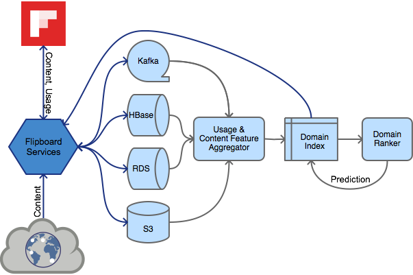
If your data pipeline is anything like ours, it will be distributed through the multiverse, covering the breadth of technologies for good measure: Kafka queues, S3 data stores, HBase, RDS, Redis, and the like. Your ML adventure will be a lot more pleasant if you can collapse the multiverse into one source of truth, ideally a memory-mapped database. Not having to deal with the complexity of a distributed system allows more focus on exploring features and classifiers.
Luckily for me, Flipboard has a custom written memory-mapped index of important article usage events that is ridiculously fast to access.

To seed the domain features, I first ran a one-time-job to aggregate all historical article events (views, likes, shares, etc.) into domain-level features, and stored them in the index for quick retrieval and updating. Then a continuous stream of real-time article usage events arrives through various pipes: Kafka queues, S3 file stores, MySQL databases, etc. These usage events are reprocessed into article features and incrementally averaged into the domain-level features, for all labeled and unlabeled domains.
Feature Engineering
Specialized knowledge about the data space goes a long way towards a successful ML application. In addition to the raw data, it is worth experimenting with more complex polynomial features that may describe a decision boundary. In our case, an obvious place to start was with article features that imply quality and engagement, like clickthrough rate, article length, quickbacks, etc.
It is important to use features that do not suffer from presentation bias. As an example, users tend to read articles that are higher in a feed as opposed to ones lower in a feed. If a recommender system boosts popular articles, a positive feedback loop occurs: popular articles are ranked higher in the feed, which are more likely to be viewed, further increasing their popularity. So popularity does not imply quality. Instead, a better feature could be something that measures follow-up actions after the user has read an article (regardless of where in the feed it was).
Feature Selection
Another consideration is reducing correlated features. For example, the time spent reading an article may be a useful feature, but it is directly correlated to length. A more informative feature is percentage of quickbacks for a domain: the portion of views with less than 10% completion. This indicates a bad experience through either pop-up ads, or users quickly realizing the content is low quality.
Many more features than the ones listed are used in practice. Feature selection helped to identify correlated and irrelevant features. We ran a fairly exhaustive search over subsets of features and picked ones that gave the best results on our validation set. The search was performed by running various classifiers on subsets of features and comparing the results.
Feature Scaling
Features can have wildly different scales. Article length for instance, ranges from 20 words to thousands of words, while quickbacks are a percentage. We can simplify the job for the classifiers by scaling all features to be in the same 0 to 1 range. This extra heuristic can also help reduce the impact of outliers. For example, if a user leaves the app open on an article, it may generate an unrealistically large view time. My rule of thumb for a reasonable scaling range was the feature average +/- 2 times the standard deviation.
Some classifiers are not affected by different feature scales, while others completely fall apart. In our case, the SVC classifier took an inordinately long time to train on unscaled features compared to other classifiers. Once the features were scaled, training got exponentially faster. Based on many experiments, scaling the features increased training speed and marginally improved the results.
Model Selection
One can spend a lifetime on this chapter of the adventure. The scikit-learn library makes it quite easy to test many families of classifiers. Thank you to all of the researchers and grad students who continue supporting this amazing library.
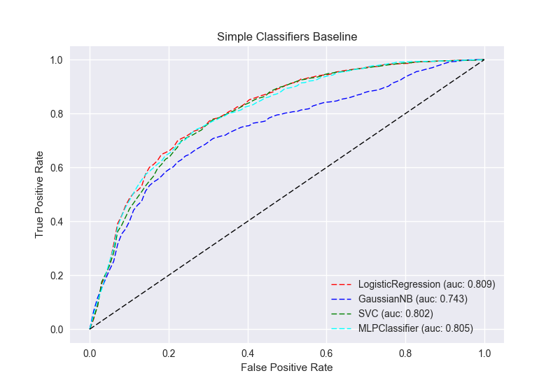
First we establish a baseline with simple models: LogisticRegression, GaussianNB, SVC, MLPClassifier. For binary classification, the Receiver Operating Characteristic (ROC) curve is the guiding light towards success. The goal is to maximize the area under the curve (auc), with a 1 being perfect classification.

These curves are the average of 5-fold cross validation train/test passes for each classifier, based on this example: ROC with cross validation.
Ensemble of Models
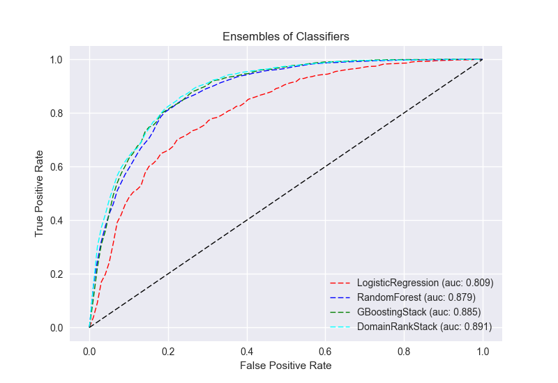
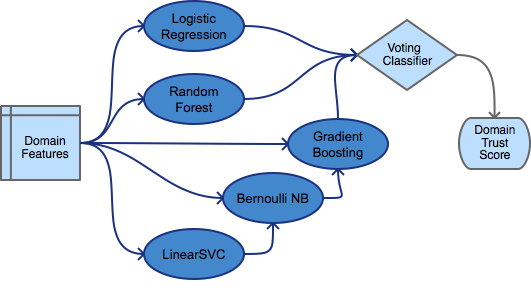
Success of the various classifiers is highly dependent on the nature of the features. Armed with the simple models as a baseline, I expanded the search to ensembles of models like RandomForest and GradientBoostingClassifier. Additionally, using TPOT: your Data Science Assistant, I was able to squeeze out a bit more prediction accuracy. It uses genetic programming to search for an optimal machine learning pipeline. TPOT resulted in this interesting GradientBoostingStack, where the results of the LinearSVC and BernoulliNB classifiers are piped into the GradientBoostingClassifier:
GBoostingStack = make_pipeline(
    make_union(VotingClassifier([("est", LinearSVC(C=20.0,
                                            dual=False,
                                            loss="squared_hinge",
                                            penalty="l1"))]),
               FunctionTransformer(lambda X: X)),

    make_union(VotingClassifier([("est", BernoulliNB(alpha=0.001,
                                            fit_prior=True))]),
               FunctionTransformer(lambda X: X)),

    GradientBoostingClassifier(learning_rate=0.1,
                               max_depth=7,
                               max_features=0.9,
                               min_samples_leaf=16,
                               min_samples_split=2,
                               subsample=0.95))

In addition to the ROC curves and overall accuracy measures, I logged all other usual metrics: Precision, Recall, F1, Specificity and Brier Score. Accuracy is not a sufficient metric, as it is biased by the test data. If accuracy is 90% and the test data is 90% positive, then the classifier may just be labeling the entire data set as positive. Specificity (true negative rate) is also important, since we are trying to catch and filter out spammers (negative labels).
Results           Accuracy |  Precision | Specificity |  Recall |      F1 |   Brier
-----------------------------------------------------------------------------------
GaussianNB           0.770 |      0.793 |       0.189 |   0.948 |   0.863 |   0.190
SVC                  0.800 |      0.798 |       0.180 |   0.990 |   0.884 |   0.134
MLPClassifier        0.812 |      0.808 |       0.232 |   0.989 |   0.890 |   0.139
LogisticRegression   0.820 |      0.833 |       0.369 |   0.958 |   0.891 |   0.132
RandomForest         0.865 |      0.881 |       0.578 |   0.953 |   0.915 |   0.102
GBoostingStack       0.870 |      0.891 |       0.619 |   0.946 |   0.918 |   0.100
DomainRankStack      0.875 |      0.887 |       0.601 |   0.959 |   0.922 |   0.097
Not all classifiers fail in the same way. Combining the 3 with the highest specificity, (RandomForest, GBoostingStack and LogisticRegression) into the DomainRankStack further boosted overall accuracy to a respectably useful 87.5%. Although specificity is slightly lower than GBoostingStack alone, the overall F1 and Brier scores have improved. Brier score is the mean squared difference between predicted probabilities and the actual outcome, so lower is better. It effectively communicates the confidence of the classifier, in addition to the prediction accuracy.

Conclusion
A “Choose Your Own ML Adventure” never truly ends. It’s a magical book, because on every re-read, new choices may appear, promising more exciting adventures. Over time, new features may be discovered, or new machine learning models may become available. Spammers may change tactics and find ways to fool a trained system. In production, our models are continuously retrained and verified as new content and data from our users and editorial team is collected.
A machine learning system is continuously sharpened, never perfected. For this reason, the Domain Ranker is just one set of “pliers” in our large tool-chest, helping to maintain the high standards of quality, truth and diversity that is expected of Flipboard.
Key Takeaways
- Build and verify the data pipeline first, separately from all else.
- If possible, aggregate the data on a single machine for much quicker experimentation.
- Engineer and scale the features.
- Garbage in/garbage out: be wary of biased and unbalanced training/test data.
- scikit-learn is really fun and incredibly useful.
- TPOT rocks.
- Ensembles of classifiers rock.
- Measure everything, rinse and repeat.
A great guide to practical ML is Martin Zinkevich’s Best Practices for ML Engineering.
Special thanks to Ben Frederickson, Arnab Bhadury, David Creemer, Mia Quagliarello and Christel van der Boom for proofreading.
Enjoyed this post? We’re hiring!